Two-stage目标检测算法将目标检测与识别的过程分为候选区域提取与目标识别两个步骤来做,由于在做具体分类识别和位置回归前多了一步候选区域提取,因此Two-stage目标检测算法的识别率和候选框精确度是比较高的,但对性能的消耗是非常巨大的。而YOLOv1作为YOLO系列算法的开山之作,创造性地提出不再预先进行候选区域(Proposal Region)的提取,而是直接将输入图片以网格的方式进行划分,由每个网格负责预测中心点落在它内部的物体。不过也正是因为缺少了Proposal Region的提取,所以相对来说回归精度要低一些。Yolo v1是端到端的,直接做预测,而不是通过候选区域提取,将目标检测问题转换为一个分类问题。
| One-stage | Two-stage |
| 优点 | 优点 |
| 推理速度快、训练快 | 精度高 |
| 背景误检率低 | 目标定位精度高 、检出率高 |
| 缺点 | 缺点 |
| 目标定位精度低 、检出率低 | 推理速度慢、训练慢 |
| 小物体检测效果差 | 背景误检率高 |
作者实现的YOLO v1版本中,输入图像的尺寸固定为448*448,在经过了24个卷积层和2个全连接层后,最后输出7*7*1024的特征图(feature map),对应了作者将原图划分为S*S个格子的思想,feature map上的每一个张量都包含了后续预测任务时所需要的高层抽象语意信息。

如图,YOLO v1将一张图片划分为S*S个格子,作者称之为栅格(grid cell)。对于一张大小为448*448的图像,经卷积层提取特征后,输出大小为7*7*1024的特征图(feature map),feature map上的每一个1*1*1024的张量就对应着原图中的一个grid cell所提取出的特征,不同的通道对应着不同的抽象语意信息。每个grid cell预测两个物体边界框(Bounding Box)以及grid cell预测的物体类别,最后通过一个NSM算法去除冗余的Bounding Box,生成检测结果。

如图, YOLO v1的网络架构为24个卷积层、4个最大池化层、2个全连接层组成,卷积和池化层部分用于特征的提取,全连接层用于预测。全连接层输出7*7*30,7*7代表原图被划分成的7*7的grid cell。
预训练模型结构定义:
import torch.nn as nn
import torchclass Convention(nn.Module):def __init__(self,in_channels,out_channels,conv_size,conv_stride,padding,need_bn = True):super(Convention,self).__init__()self.conv = nn.Conv2d(in_channels, out_channels, conv_size, conv_stride, padding, bias=False if need_bn else True)self.leaky_relu = nn.LeakyReLU(inplace=True,negative_slope=1e-1)self.need_bn = need_bnif need_bn:self.bn = nn.BatchNorm2d(out_channels)def forward(self, x):return self.bn(self.leaky_relu(self.conv(x))) if self.need_bn else self.leaky_relu(self.conv(x))def weight_init(self):for m in self.modules():if isinstance(m, nn.Conv2d):torch.nn.init.kaiming_normal_(m.weight.data)elif isinstance(m, nn.BatchNorm2d):m.weight.data.fill_(1)m.bias.data.zero_()class YOLO_Feature(nn.Module):def __init__(self, classes_num=80):super(YOLO_Feature,self).__init__()self.Conv_Feature = nn.Sequential(Convention(3, 64, 7, 2, 3),nn.MaxPool2d(2, 2),Convention(64, 192, 3, 1, 1),nn.MaxPool2d(2, 2),Convention(192, 128, 1, 1, 0),Convention(128, 256, 3, 1, 1),Convention(256, 256, 1, 1, 0),Convention(256, 512, 3, 1, 1),nn.MaxPool2d(2, 2),Convention(512, 256, 1, 1, 0),Convention(256, 512, 3, 1, 1),Convention(512, 256, 1, 1, 0),Convention(256, 512, 3, 1, 1),Convention(512, 256, 1, 1, 0),Convention(256, 512, 3, 1, 1),Convention(512, 256, 1, 1, 0),Convention(256, 512, 3, 1, 1),Convention(512, 512, 1, 1, 0),Convention(512, 1024, 3, 1, 1),nn.MaxPool2d(2, 2),)self.Conv_Semanteme = nn.Sequential(Convention(1024, 512, 1, 1, 0),Convention(512, 1024, 3, 1, 1),Convention(1024, 512, 1, 1, 0),Convention(512, 1024, 3, 1, 1),)self.avg_pool = nn.AdaptiveAvgPool2d(1)self.linear = nn.Linear(1024, classes_num)def forward(self, x):x = self.Conv_Feature(x)x = self.Conv_Semanteme(x)x = self.avg_pool(x)# batch_size * channel * width * heightx = x.permute(0, 2, 3, 1)x = torch.flatten(x, start_dim=1, end_dim=3)x = self.linear(x)return x# 定义权值初始化def initialize_weights(self):for m in self.modules():if isinstance(m, nn.Conv2d):torch.nn.init.kaiming_normal_(m.weight.data)elif isinstance(m, nn.BatchNorm2d):m.weight.data.fill_(1)m.bias.data.zero_()elif isinstance(m, nn.Linear):torch.nn.init.kaiming_normal_(m.weight.data)m.bias.data.zero_()elif isinstance(m, Convention):m.weight_init()
注:笔者此处并对YOLOv1前20个普通卷积改进为Conv+BN层,是为了利用BN层来加速网络的收敛。时至今日,BN+Residual已经成为了CNN进行特征提取的标配,当然值得注意的是,在GAN-generator中,更为合适的是LayerNormal,不同的领域有各自适应的方法。
使用COCO数据集中的目标进行预训练(当然有条件的还是建议使用ImageNet预训练):
注:笔者先前使用过ImageNet-Tiny数据集训练,发现效果很差,检查数据集后发现Tiny系数据集的实际待分类目标占整幅图像的比例很低,而在YOLOv1的网络中存在全局平均池化,因此会加剧收敛出现问题。举例来说,假设都是鱼的种类,一幅图片是一只占图像比例很大的鱼,另一幅图片是一个人手中抱着一只鱼,在全局池化后,后者中混入了较多了人类的特征,我们在当前将其往鱼的类别收敛,那么当我们遇到分类目标为人的图片后,又需要朝着将其分类为人的目标迭代,因此网络将一直在人是鱼/人是人两种决策中摇摆,无法收敛。
所以笔者采用的替代方案为,利用现有的COCO数据集的bounding box标注,将拥有最小杂信息的图像区域框选出来,用这部分图像区域进行训练。
好处:杂项信息更少,网络便于训练收敛
坏处:图像简单导致任务变得简单,同时网络可能学不会利用背景辅助判断物体
注:笔者对于训练过程使用了数据增强,对于验证过程则不用数据增强。 训练过程: 如图,由于作者使用了VOC数据集(20个类别)来测试并测试YOLO v1,所以预测输出的张量中,前面两个5维分别表示两个Bounding Box的物体置信度以及两个box各自的中心坐标及宽高,后面的20维对应了20种类别各自的概率。 IOU:(区域交并比) 在目标检测领域,IoU是一个重要指标,通过两个box的交集和并集的面积值比值来衡量两个boxes的接近程度(重叠程度)。 矩形交集计算:223. 矩形面积_The Shawshank Redemption-CSDN博客 置信度:作者采用了同时考虑有无物体以及定位准确度的方式 预测输出的结果我们使用sigmod函数将输出压缩在(0,1),在制作Ground Truth时,我们根据上述约定直接计算即可。 使用VOC数据集进行目标检测的训练 用于目标检测的YOLOv1网络结构: VOC目标检测数据集类: [注]:在YOLO v1中,每一个grid cell虽然预测两个bounding box,但是最终只有一个是有效的,最多检测7*7*1=49个物体。为简单起见,在本人的实现中,对于多个物体的重心落于同一个grid cell的情况(概率非常低),采用的方式是选择最后一个确定是该方格负责的物体。mask操作是为了利用一部分显存实现快速计算正负样本损失。 损失函数是深度学习网络模型非常重要的“指挥棒”,负责引导整体网络的任务和学习方向,通过对预测样本和真实样本的误差进行反向传播来指导网络进行参数的调整学习。 我们将含有物体的Bounding Box当作正样本,将不含有物体的Bounding Box当作负样本。在实际的实现上,通过Bounding Box与真实的物体边界框(Ground Truth)的IoU值来判定正负样本,将与Ground Truth拥有最大IoU值的box当作正样本,其余的box作为负样本。 整个YOLO v1算法的损失函数就包含分别关于正样本(负责预测物体的Bounding Box)和负样本(负责预测物体的Bounding Box)两部分,正样本置信度为1,负样本置信度为0,正样本的损失包含置信度损失、边框回归损失和类别损失,而负样本损失只有置信度损失。 [注]:这边解释一下,因为我们预先设置好了S*S*B个Bounding Box,但是有可能存在一些Bounding Box是完全没有预测到目标的,那些预测到目标的Bounding Box就是正样本,没有预测到目标的就是负样本。在作者创作YOLO v1的那个年代,用于目标检测的数据还没有特别密集的目标的情况,因此存在较多的负样本。 YOLO v1的损失由5个部分组成,均使用均方差损失: (1) 第一部分为正样本中心点坐标的损失,引入 [注]:对于YOLOv1来说,正负样本的归属取决于在预测阶段 预测框与真实框的IoU值,若一个物体落在某个cell内,那么由这个cell预测出的两个box中,与真实框拥有更大IoU值的box负责拟合,即作为正样本,另一个即为负样本。 另外,在最初的时候,先冻结backbone部分训练10个epoch,先训练出预测部分,然后再让预测部分与特征提取部分共同训练。 通常来说,目标检测算法的最终输出结果是很多的Bounding Box用于预测目标,常用做法是将所有的Box通过非极大值抑制(NMS)算法去除冗余,保留效果最好的。 算法 NMS算法 输入:Bounding Box的集合p、IoU阈值、置信度阈值。 输出:去除冗余的Bounding box集合q。 1.去除集合p中置信度低于置信度阈值的Bounding Box。 2.在集合p中选取拥有最大置信度的Box,移出集合p并加入集合q,并将p中剩余的Bounding Box与该box计算IOU值,去除那些与该Box的IOU值超过阈值的Bounding Box。 3.重复步骤2,直到集合p为空 4.输出集合q,为所求的结果集合。 NMS: ①在3*3的卷积后接上一个通道数低的1*1的卷积,用于进行特征的通道压缩,降低计算量;同时多一层的卷积也提升了模型的非线性表达能力。 ②在训练中使用Dropout和数据增强的方式来防止网络过拟合。 ③并没有引入Anchor机制,而是直接在每个区域进行框的大小与位置信息的预测,利用区域本身携带的位置信息和被检测物体尺度处于网络可以回归范围之内的特性将目标检测问题转化为一个回归问题。 ④YOLO v1将物体类别与物体置信度分开预测,简化了问题,实验证明YOLO v1背景误检率要低于Fast R-CNN,YOLO v1的误差主要来源是定位误差,如图4-7所示: ①每一个区域只预测两个框,并且共用同一个类别向量,这导致YOLO v1只能检测有限个物体,并且对于小物体和距离相近的物体的检测效果并不好,而实际的情况下,预测的7*7*2=98个bounding box中,最多只有49个是有效的,也就是说YOLO v1对于一张图片最多预测49个物体。 ②由于没有引入Anchor机制,而是直接从数据中学习并进行预测,故很难泛化到新的、不常见的宽高比例的目标的检测中,所以模型对于新的或者并不常见宽高比例的物体检测效果并不好。另外,由于下采样率比较大,对于边框的回归精度也不高。 ③在v1的损失函数设计中,大物体和小物体的定位损失权重一样,这将会导致同等比例的定位误差,大物体的损失会比小物体大,小物体的损失在总损失中占比较小,然而实际上,小边界框的小误差对IoU的影响比大边界框要大得多,会导致定位的不准确,但是作者也是知道的,只不过为了保持YOLO v1简单的特性,作者的处理方式是使用对尺度开方,依此提高小物体尺度损失的相对权重。 相较于DPM等传统方法而言,YOLO有更高的精度;相较于以Fast R-CNN为代表的一系列的Two-stage算法,YOLO的精度稍有逊色,但是FPS达到了完全碾压的地步,兼顾了实时性和精度,使得工业上用深度学习做目标检测成为可能。 为了避免卷积的输出reshape为普通张量导致的特征图错乱的问题,因此本人还提出一种全卷积结构用来实验对YOLO V1的推理能力进行优化,结合1*1的卷积进行特征压缩,而不是直接降采样,依此来提高有效的特征保留。 在深度学习中,学习率在初期往往很大,一是可以用来加快训练,二是可以冲出鞍点和一些局部最优点;而在后期,网络稳定收敛到某个最小值时(实际上可能还是局部最小,因为深度学习不是一个凸优化问题,因此我们不太可能正好找到那个最优解,但是我们可以通过学习算法获得一个较为优秀的解),为了避免网络发散,同时防止网络在最小值附近不断震荡,而应该调小学习率,让网络顺着那个最小值的方向进行下降。 为了更好地监控网络的训练情况,本人在项目中引入了Tensorboard功能。 本人打算先复现一个功能上还算完善的网络,后期还会加入数据集扩充等功能,并继续优化网络的计算速度以及显存占用~~ 全卷积网络收敛情况 YOLO V1原网络收敛情况 项目复现github地址:经过几版本重构后,原仓库太大导致上传太慢,现全部转移至新仓库 GitHub - ProgrammerZhujinming/YOLOimport cv2
import os
import time
import random
import imagesize
import numpy as np
from utils import image
from torch.utils.data import Dataset
import torchvision.transforms as transformsclass coco_classify_dataset(Dataset):def __init__(self,imgs_path = "../DataSet/COCO2017/Train/Imgs", txts_path = "../DataSet/COCO2017/Train/Labels", is_train = True, edge_threshold=200, class_num=80, input_size=256): # input_size:输入图像的尺度img_names = os.listdir(txts_path)self.is_train = is_trainself.transform_common = transforms.Compose([transforms.ToTensor(), # height * width * channel -> channel * height * widthtransforms.Normalize(mean=(0.408, 0.448, 0.471), std=(0.242, 0.239, 0.234)) # 归一化后.不容易产生梯度爆炸的问题])self.input_size = input_sizeself.train_data = [] # [img_path,[[coord, class_id]]]for img_name in img_names:img_path = os.path.join(imgs_path, img_name.replace(".txt", ".jpg"))txt_path = os.path.join(txts_path, img_name)coords = []with open(txt_path, 'r') as label_txt:for label in label_txt:label = label.replace("\n", "").split(" ")class_id = int(label[4])if class_id >= class_num:continuexmin = round(float(label[0]))ymin = round(float(label[1]))xmax = round(float(label[2]))ymax = round(float(label[3]))if (xmax - xmin) #------0.common variable definition------
import torch
import argparse
import torch.nn as nn
from tqdm import tqdm
import torch.optim as optim
from utils.model import accuracy
from tensorboardX import SummaryWriter
from torch.utils.data import DataLoader
from utils.model import feature_map_visualize
from YOLO.PreTrain.YOLO_Feature import YOLO_Feature
from YOLO.PreTrain.COCO_Classify_DataSet import coco_classify_dataset
if torch.cuda.is_available():device = torch.device('cuda:0')torch.backends.cudnn.benchmark = True
else:device = torch.device('cpu')if __name__ == "__main__":# 1.training parametersparser = argparse.ArgumentParser(description="YOLO_Feature train config")parser.add_argument('--batch_size', type=int, help="YOLO_Feature train batch_size", default=32)parser.add_argument('--num_workers', type=int, help="YOLO_Feature train num_worker num", default=4)parser.add_argument('--lr', type=float, help="lr", default=3e-4)parser.add_argument('--weight_decay', type=float, help="weight_decay", default=0.0005)parser.add_argument('--epoch_num', type=int, help="YOLO_Feature train epoch_num", default=200)parser.add_argument('--epoch_interval', type=int, help="save YOLO_Feature interval", default=10)parser.add_argument('--class_num', type=int, help="YOLO_Feature train class_num", default=80)parser.add_argument('--train_imgs', type=str, help="YOLO_Feature train train_imgs", default="../../DataSet/COCO2017/Train/Imgs")parser.add_argument('--train_labels', type=str, help="YOLO_Feature train train_labels", default="../../DataSet/COCO2017/Train/Labels")parser.add_argument('--val_imgs', type=str, help="YOLO_Feature train val_imgs", default="../../DataSet/COCO2017/Val/Imgs")parser.add_argument('--val_labels', type=str, help="YOLO_Feature train val_labels", default="../../DataSet/COCO2017/Val/Labels")parser.add_argument('--grad_visualize', type=bool, help="YOLO_Feature train grad visualize", default=False)parser.add_argument('--feature_map_visualize', type=bool, help="YOLO_Feature train feature map visualize", default=False)parser.add_argument('--restart', type=bool, help="YOLO_Feature train from zeor?", default=True)parser.add_argument('--pre_weight_file', type=str, help="YOLO_Feature pre weight path", default="./weights/YOLO_Feature_20.pth")args = parser.parse_args()batch_size = args.batch_sizenum_workers = args.num_workersepoch_num = args.epoch_numepoch_interval = args.epoch_intervalclass_num = args.class_numif args.restart == True:lr = args.lrparam_dict = {}epoch = 0epoch_val_loss_min = 999999999else:param_dict = torch.load(args.pre_weight_file, map_location=torch.device("cpu"))optimal_dict = param_dict['optimal']epoch = param_dict['epoch']epoch_val_loss_min = param_dict['epoch_val_loss_min']# 2.datasettrain_dataSet = coco_classify_dataset(imgs_path=args.train_imgs,txts_path=args.train_labels, is_train=True, edge_threshold=200)val_dataSet = coco_classify_dataset(imgs_path=args.val_imgs,txts_path=args.val_labels, is_train=False, edge_threshold=200)# 3-4.network - optimizeryolo_feature = YOLO_Feature(classes_num=class_num)if args.restart == True:yolo_feature.initialize_weights()optimizer = optim.Adam(params=yolo_feature.parameters(), lr=args.lr, weight_decay=args.weight_decay)else:yolo_feature.load_state_dict(param_dict['model'])optimizer = param_dict['optimizer']yolo_feature.to(device=device, non_blocking=True)# 5.lossloss_function = nn.CrossEntropyLoss().to(device=device)# 6.train and recordinput_size = 256writer = SummaryWriter(logdir='./log', filename_suffix=' [' + str(epoch) + '~' + str(epoch + epoch_interval) + ']')while epoch 3.YOLOv1输出结构


def iou(self, box1, box2): # 计算两个box的IoU值# box: lx-左上x ly-左上y rx-右下x ry-右下y 图像向右为y 向下为x# 1. 获取交集的矩形左上和右下坐标interLX = max(box1[0],box2[0])interLY = max(box1[1],box2[1])interRX = min(box1[2],box2[2])interRY = min(box1[3],box2[3])# 2. 计算两个矩形各自的面积Area1 = (box1[2] - box1[0]) * (box1[3] - box1[1])Area2 = (box2[2] - box2[0]) * (box2[3] - box2[1])# 3. 不存在交集if interRX 
import torch
import torch.nn as nn
from YOLO.PreTrain.YOLO_Feature import Conventionclass YOLOv1(nn.Module):def __init__(self,B=2,classes_num=20):super(YOLOv1,self).__init__()self.B = Bself.classes_num = classes_numself.Conv_Feature = nn.Sequential(Convention(3, 64, 7, 2, 3),nn.MaxPool2d(2, 2),Convention(64, 192, 3, 1, 1),nn.MaxPool2d(2, 2),Convention(192, 128, 1, 1, 0),Convention(128, 256, 3, 1, 1),Convention(256, 256, 1, 1, 0),Convention(256, 512, 3, 1, 1),nn.MaxPool2d(2, 2),Convention(512, 256, 1, 1, 0),Convention(256, 512, 3, 1, 1),Convention(512, 256, 1, 1, 0),Convention(256, 512, 3, 1, 1),Convention(512, 256, 1, 1, 0),Convention(256, 512, 3, 1, 1),Convention(512, 256, 1, 1, 0),Convention(256, 512, 3, 1, 1),Convention(512, 512, 1, 1, 0),Convention(512, 1024, 3, 1, 1),nn.MaxPool2d(2, 2),)self.Conv_Semanteme = nn.Sequential(Convention(1024, 512, 1, 1, 0),Convention(512, 1024, 3, 1, 1),Convention(1024, 512, 1, 1, 0),Convention(512, 1024, 3, 1, 1),)self.Conv_Back = nn.Sequential(Convention(1024, 1024, 3, 1, 1, need_bn=False),Convention(1024, 1024, 3, 2, 1, need_bn=False),Convention(1024, 1024, 3, 1, 1, need_bn=False),Convention(1024, 1024, 3, 1, 1, need_bn=False),)self.Fc = nn.Sequential(nn.Linear(7*7*1024,4096),nn.LeakyReLU(inplace=True, negative_slope=1e-1),nn.Linear(4096,7 * 7 * (B*5 + classes_num)),)self.sigmoid = nn.Sigmoid()self.softmax = nn.Softmax(dim=3)def forward(self, x):x = self.Conv_Feature(x)x = self.Conv_Semanteme(x)x = self.Conv_Back(x)# batch_size * channel * height * weight -> batch_size * height * weight * channelx = x.permute(0, 2, 3, 1)x = torch.flatten(x, start_dim=1, end_dim=3)x = self.Fc(x)x = x.view(-1, 7, 7, (self.B * 5 + self.classes_num))#print("x seg:{}".format(x[:,:,:,0 : self.B * 5]))bnd_coord = self.sigmoid(x[:,:,:,0 : self.B * 5])#print("bnd_coord:{}".format(bnd_coord))bnd_cls = self.softmax(x[:,:,:, self.B * 5 : ])bnd = torch.cat([bnd_coord, bnd_cls], dim=3)#x = self.sigmoid(x.view(-1,7,7,(self.B * 5 + self.classes_num)))#x[:,:,:, 0 : self.B * 5] = self.sigmoid(x[:,:,:, 0 : self.B * 5])#x[:,:,:, self.B * 5 : ] = self.softmax(x[:,:,:, self.B * 5 : ])return bnd# 定义权值初始化def initialize_weights(self, net_param_dict):for name, m in self.named_modules():if isinstance(m, nn.Conv2d):torch.nn.init.kaiming_normal_(m.weight.data)elif isinstance(m, nn.BatchNorm2d):m.weight.data.fill_(1)m.bias.data.zero_()elif isinstance(m, nn.Linear):torch.nn.init.kaiming_normal_(m.weight.data)m.bias.data.zero_()elif isinstance(m, Convention):m.weight_init()self_param_dict = self.state_dict()for name, layer in self.named_parameters():if name in net_param_dict:self_param_dict[name] = net_param_dict[name]self.load_state_dict(self_param_dict)from torch.utils.data import Dataset
import os
import cv2
import xml.etree.ElementTree as ET
import torchvision.transforms as transforms
import numpy as np
import random
import torch
from utils import imageclass VOC_Detection_Set(Dataset):def __init__(self, imgs_path="../DataSet/VOC2007+2012/Train/JPEGImages",annotations_path="../DataSet/VOC2007+2012/Train/Annotations",classes_file="../DataSet/VOC2007+2012/class.data", is_train = True, class_num=20,label_smooth_value=0.05, input_size=448, grid_size=64, loss_mode="mse"): # input_size:输入图像的尺度self.label_smooth_value = label_smooth_valueself.class_num = class_numself.imgs_name = os.listdir(imgs_path)self.input_size = input_sizeself.grid_size = grid_sizeself.is_train = is_trainself.transform_common = transforms.Compose([transforms.ToTensor(), # height * width * channel -> channel * height * widthtransforms.Normalize(mean=(0.408, 0.448, 0.471), std=(0.242, 0.239, 0.234)) # 归一化后.不容易产生梯度爆炸的问题])self.imgs_path = imgs_pathself.annotations_path = annotations_pathself.class_dict = {}self.loss_mode = loss_modeclass_index = 0with open(classes_file, 'r') as file:for class_name in file:class_name = class_name.replace('\n', '')self.class_dict[class_name] = class_index # 根据类别名制作索引class_index = class_index + 1def __getitem__(self, item):img_path = os.path.join(self.imgs_path, self.imgs_name[item])annotation_path = os.path.join(self.annotations_path, self.imgs_name[item].replace(".jpg", ".xml"))img = cv2.imread(img_path)tree = ET.parse(annotation_path)annotation_xml = tree.getroot()objects_xml = annotation_xml.findall("object")coords = []for object_xml in objects_xml:bnd_xml = object_xml.find("bndbox")class_name = object_xml.find("name").textif class_name not in self.class_dict: # 不属于我们规定的类continuexmin = round((float)(bnd_xml.find("xmin").text))ymin = round((float)(bnd_xml.find("ymin").text))xmax = round((float)(bnd_xml.find("xmax").text))ymax = round((float)(bnd_xml.find("ymax").text))class_id = self.class_dict[class_name]coords.append([xmin, ymin, xmax, ymax, class_id])coords.sort(key=lambda coord : (coord[2] - coord[0]) * (coord[3] - coord[1]) )if self.is_train:transform_seed = random.randint(0, 4)if transform_seed == 0: # 原图img, coords = image.resize_image_with_coords(img, self.input_size, self.input_size, coords)img = self.transform_common(img)elif transform_seed == 1: # 缩放+中心裁剪img, coords = image.center_crop_with_coords(img, coords)img, coords = image.resize_image_with_coords(img, self.input_size, self.input_size, coords)img = self.transform_common(img)elif transform_seed == 2: # 平移img, coords = image.transplant_with_coords(img, coords)img, coords = image.resize_image_with_coords(img, self.input_size, self.input_size, coords)img = self.transform_common(img)else: # 曝光度调整img, coords = image.resize_image_with_coords(img, self.input_size, self.input_size, coords)img = image.exposure(img, gamma=0.5)img = self.transform_common(img)else:img, coords = image.resize_image_with_coords(img, self.input_size, self.input_size, coords)img = self.transform_common(img)ground_truth, ground_mask_positive, ground_mask_negative = self.getGroundTruth(coords)return img, [ground_truth, ground_mask_positive, ground_mask_negative, img_path]#ground_truth, ground_mask_positive, ground_mask_negative = self.getGroundTruth(coords)# 通道变化方法: img = img[:, :, ::-1]#return img, ground_truth, ground_mask_positive, ground_mask_negativedef __len__(self):return len(self.imgs_name)def getGroundTruth(self, coords):feature_size = self.input_size // self.grid_size#ground_mask_positive = np.zeros([feature_size, feature_size, 1], dtype=bool)#ground_mask_negative = np.ones([feature_size, feature_size, 1], dtype=bool)ground_mask_positive = np.full(shape=(feature_size, feature_size, 1), fill_value=False, dtype=bool)ground_mask_negative = np.full(shape=(feature_size, feature_size, 1), fill_value=True, dtype=bool)if self.loss_mode == "mse":ground_truth = np.zeros([feature_size, feature_size, 10 + self.class_num + 2])else:ground_truth = np.zeros([feature_size, feature_size, 10 + 1])for coord in coords:xmin, ymin, xmax, ymax, class_id = coordground_width = (xmax - xmin)ground_height = (ymax - ymin)center_x = (xmin + xmax) / 2center_y = (ymin + ymax) / 2index_row = (int)(center_y * feature_size)index_col = (int)(center_x * feature_size)# 分类标签 label_smoothif self.loss_mode == "mse":# 转化为one_hot编码 对one_hot编码做平滑处理class_list = np.full(shape=self.class_num, fill_value=1.0, dtype=float)deta = 0.01class_list = class_list * deta / (self.class_num - 1)class_list[class_id] = 1.0 - detaelif self.loss_mode == "cross_entropy":class_list = [class_id]else:raise Exception("the loss mode can't be support now!")# 定位数据预设ground_box = [center_x * feature_size - index_col, center_y * feature_size - index_row,ground_width, ground_height, 1,round(xmin * self.input_size), round(ymin * self.input_size),round(xmax * self.input_size), round(ymax * self.input_size),round(ground_width * self.input_size * ground_height * self.input_size)]ground_box.extend(class_list)ground_box.extend([index_col, index_row])ground_truth[index_row][index_col] = np.array(ground_box)ground_mask_positive[index_row][index_col] = Trueground_mask_negative[index_row][index_col] = Falsereturn ground_truth, torch.BoolTensor(ground_mask_positive), torch.BoolTensor(ground_mask_negative)4. YOLO v1 损失函数

5. YOLOv1预测结果处理--NMS算法
import numpy as np# 这边要求的bounding_boxes为处理后的实际的样子
def NMS(bounding_boxes,confidence_threshold,iou_threshold):# boxRow : x y dx dy c# 1. 初步筛选,先把grid cell预测的两个bounding box取出置信度较高的那个boxes = []for boxRow in bounding_boxes:# grid cell预测出的两个box,含有物体的置信度没有达到阈值if boxRow[4] 6. YOLO v1分析
1.YOLO v1网络优势

2.YOLO v1缺陷分析
3.YOLO v1与其他网络的性能对比:

7.个人训练优化策略(已删除,基本按照YOLOv1论文复现)
1.全卷积结构
2.多步长调整学习率
3.Tensorboard监控训练
4.后期准备
5.当前网络情况


![[echarts] 同指标对比柱状图相关的知识介绍及应用示例](https://img7.php1.cn/3cdc5/c7bc/ae9/d860963d11bbd36d.jpeg)

 京公网安备 11010802041100号 | 京ICP备19059560号-4 | PHP1.CN 第一PHP社区 版权所有