本文是在模仿中精进数据分析与可视化系列的第一期——颗粒物浓度时空变化趋势(Mann–Kendall Test),主要目的是参考其他作品模仿学习进而提高数据分析与可视化的能力,如果有问题和建议,欢迎在评论区指出。若有其他想要看的作品,也欢迎在评论区留言并给出相关信息。
所用数据和代码的下载地址如下:
链接:https://pan.baidu.com/s/1IixHE9aPf1u9qFkdAdHQaA
提取码:hmq2
复制这段内容后打开百度网盘手机App,操作更方便哦
简介
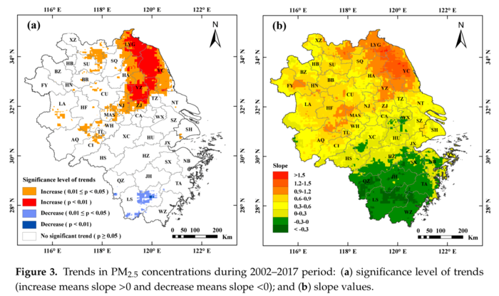
本次要模仿的作品来自论文Investigating the Impacts of Urbanization on PM2.5 Pollution in the Yangtze River Delta of China: A Spatial Panel Data Approach,研究区域为上海、安徽、浙江和江苏,所用数据为 2002–2017该区域PM2.5浓度栅格数据,数据来源于 Dalhousie University Atmospheric Composition Analysis Group开发的年均PM2.5数据集V4.CH.03,空间分辨率为0.01°×0.1°(原论文采用数据的空间分辨率为1km×1km,但我在该网站上找不到,可能是不提供下载了)。
数据下载和处理
数据下载格式为.asc,使用arcpy将其转为.tif格式,所用代码如下。
# -*- coding: utf-8 -*-

import arcpy
import os

inpath = "./ASCII" #待转换的栅格的存储路径,会转换该路径下的所有栅格
outpath = "./TIF" #输出栅格的路径,最好是空路径
filetype = "FLOAT"

print "Starting Convert!"
for filename in os.listdir(inpath):
    if filename.endswith(".asc"):
        filepath = os.path.join(inpath, filename)
        outfilepath = os.path.join(outpath, filename.replace(".asc", ".tif"))
        arcpy.ASCIIToRaster_conversion(filepath, outfilepath, filetype)
print "Convert Over!"
Mann–Kendall趋势分析
Mann–Kendall趋势分析的具体计算方法这里不再赘述,原文作者采用R语言的trend package计算的,本文采用python的pymannkendall计算,github项目地址为https://github.com/mmhs013/pyMannKendall。
原文的趋势分析包括两部分,一部分是计算slope值,slope值为正,则表明具有上升的趋势,反之亦然;另一部分是计算p值,p值越小趋势越显著,0.01sens_slope和original_test函数计算,pymannkendall的简单用法介绍如下。
A quick example of pyMannKendall usage is given below. Several more examples are provided here.
import numpy as np
import pymannkendall as mk

# Data generation for analysis
data = np.random.rand(360,1)

result = mk.original_test(data)
print(result)
Output are like this:
Mann_Kendall_Test(trend='no trend', h=False, p=0.9507221701045581, z=0.06179991635055463, Tau=0.0021974620860414733, s=142.0, var_s=5205500.0, slope=1.0353584906597959e-05, intercept=0.5232692553379981)
Whereas, the output is a named tuple, so you can call by name for specific result:
print(result.slope)
or, you can directly unpack your results like this:
trend, h, p, z, Tau, s, var_s, slope, intercept = mk.original_test(data)
计算并保存结果
这里依然使用arcpy作为分析计算的工具,所用代码如下。
pymannkendall较为臃肿,计算速度很慢(全部计算用了十几分钟),并且暂不支持numba加速,有需要大量计算的可根据其源码重新编写函数,实现numba加速,如本文的get_slope函数,在使用numba加速后计算pvalues仅需4秒,使用pymannkendall的sens_test则需要几分钟的时间。
# -*- coding: utf-8 -*-

import arcpy
import os
from glob import glob
import numpy as np
import pymannkendall as mk

inpath = r"./TIF" #.tif文件的保存路径
p_path = r"./pvalues.tif" #p-values的输出路径
slope_path = r"./slopes.tif" #slopes的输出路径
trend_path = r"./trends.tif" #原图左图中不同的趋势
border_path = r"./Shapefiles/border.shp" #研究区域

# 获取2002-2017年的栅格数据的路径
def get_raster_paths(inpath):
    paths = []
    for year in range(2002, 2018):
        year_path = glob(os.path.join(inpath, "*"+str(year)+"*.tif"))
        if year_path:
            paths.append(year_path[0])
        else:
            print "can't find raster of {} year!".format(year)
    return paths

# 裁剪栅格,并将结果转为numpy数组
def clip_raster_to_array(paths, border):
    out_image = arcpy.sa.ExtractByMask(paths[0], border)
    # 掩膜提取
    x_cell_size, y_cell_size = out_image.meanCellWidth, out_image.meanCellHeight #x,y方向的像元大小
    ExtentXmin, ExtentYmin = out_image.extent.XMin, out_image.extent.YMin #取x,y坐标最小值
    lowerLeft = arcpy.Point(ExtentXmin, ExtentYmin) #取得数据起始点范围
    noDataValue = out_image.noDataValue #取得数据的noData值
    out_image = arcpy.RasterToNumPyArray(out_image) #将栅格转为numpy数组
    out_image[out_image==noDataValue] = np.NAN #将数组中的noData值设为nan
    arrays = np.full(shape=(len(paths), out_image.shape[0], out_image.shape[1]),
                     fill_value=np.NAN, dtype=out_image.dtype)
    arrays[0] = out_image

    for i in range(1, len(paths)):
        out_image = arcpy.sa.ExtractByMask(paths[i], border)
        out_image = arcpy.RasterToNumPyArray(out_image)
        out_image[out_image==noDataValue] = np.NAN
        arrays[i] = out_image

    return arrays, (lowerLeft, x_cell_size, y_cell_size, noDataValue)

def array_to_raster(path, data, rasterInfo):
    new_raster = arcpy.NumPyArrayToRaster(data, *rasterInfo) #数组转栅格
    new_raster.save(path) #保存栅格

# 计算slope值
def get_slope(x):
    if np.isnan(x).any():
        return np.NAN
    idx = 0
    n = len(x)
    d = np.ones(int(n*(n-1)/2))

    for i in range(n-1):
        j = np.arange(i+1,n)
        d[idx : idx + len(j)] = (x[j] - x[i]) / (j - i)
        idx = idx + len(j)

    return np.median(d)

# 计算p值
def get_pvalue(x):
    if np.isnan(x).any():
        return np.NAN
    result = mk.original_test(x)
    return result.p

paths = get_raster_paths(inpath)
arrays, rasterinfo = clip_raster_to_array(paths, border_path)
print "clip raster to array over!"

slopes = np.apply_along_axis(get_slope, 0, arrays)
print "calculate p-value over!"
pvalues = np.apply_along_axis(get_pvalue, 0, arrays)
print "calculate slope over!"

#计算有显著和非常显著趋势的区域
trends = np.full(shape=slopes.shape, fill_value=np.NaN)
trends[~np.isnan(slopes)] = 0 #不显著的区域设为0
trends[(slopes>0) & ((0.010) & (pvalues<0.01)] = 2 #显著增加的区域设为2
trends[(slopes<0) & ((0.01
结果绘图
由于QGIS软件打开和一些相关操作的速度都要比ArcGIS快的多,而且QGIS内置的取色器的功能也方便绘图时设置颜色,因此本文使用QGIS绘制结果图,如下图所示。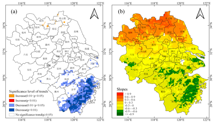


 京公网安备 11010802041100号