F:\python_enter_anaconda510\Lib\site-packages\tensorflow\python\keras\datasets
https://s3.amazonaws.com/img-datasets/mnist.npz
from __future__ import absolute_import
from __future__ import division
from __future__ import print_function

from ..utils.data_utils import get_file
import numpy as np

def load_data(path='mnist.npz'):
    """Loads the MNIST dataset.
    # Arguments
        path: path where to cache the dataset locally
            (relative to ~/.keras/datasets).
    # Returns
        Tuple of Numpy arrays: `(x_train, y_train), (x_test, y_test)`.
    """
    path = 'E:/Data/Mnist/mnist.npz' #此处的path为你刚刚防止mnist.py的目录。注意斜杠
    f = np.load(path)
    x_train, y_train = f['x_train'], f['y_train']
    x_test, y_test = f['x_test'], f['y_test']
    f.close()
    return (x_train, y_train), (x_test, y_test)
补充:Keras MNIST 手写数字识别数据集
1 导入相关的模块
import keras
import numpy as np
from keras.utils import np_utils
import os
from keras.datasets import mnist
2 第一次进行Mnist 数据的下载
(X_train_image ,y_train_image),(X_test_image,y_test_image) = mnist.load_data()
第一次执行 mnist.load_data() 方法 ,程序会检查用户目录下是否已经存在 MNIST 数据集文件 ,如果没有,就会自动下载 . (所以第一次运行比较慢) .
3 查看已经下载的MNIST 数据文件

4 查看MNIST数据
print('train data = ' ,len(X_train_image)) #
print('test data = ',len(X_test_image))
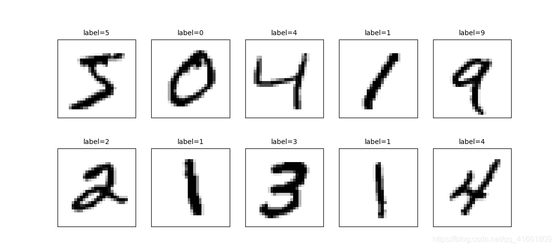
1 训练集是由 images 和 label 组成的 , images 是数字的单色数字图像 28 x 28 的 , label 是images 对应的数字的十进制表示 .
2 显示数字的图像
import matplotlib.pyplot as plt
def plot_image(image):
    fig = plt.gcf()
    fig.set_size_inches(2,2)  # 设置图形的大小
    plt.imshow(image,cmap='binary') # 传入图像image ,cmap 参数设置为 binary ,以黑白灰度显示
    plt.show()
3 查看训练数据中的第一个数据
plot_image(x_train_image[0])

查看对应的标记(真实值)
print(y_train_image[0])
运行结果 : 5
上面我们只显示了一组数据的图像 , 下面将显示多组手写数字的图像展示 ,以便我们查看数据 .
def plot_images_labels_prediction(images, labels,
                                  prediction, idx, num=10):
    fig = plt.gcf()
    fig.set_size_inches(12, 14) # 设置大小
    if num > 25: num = 25
    for i in range(0, num):
        ax = plt.subplot(5, 5, 1 + i)# 分成 5 X 5 个子图显示, 第三个参数表示第几个子图
        ax.imshow(images[idx], cmap='binary')
        title = "label=" + str(labels[idx])
        if len(prediction) > 0: # 如果有预测值
            title += ",predict=" + str(prediction[idx])

        ax.set_title(title, fOntsize=10)
        ax.set_xticks([])
        ax.set_yticks([])
        idx += 1
    plt.show()
plot_images_labels_prediction(x_train_image,y_train_image,[],0,10)
查看测试集 的手写数字前十个
plot_images_labels_prediction(x_test_image,y_test_image,[],0,10)

feature (数字图像的特征值) 数据预处理可分为两个步骤:
(1) 将原本的 288 X28 的数字图像以 reshape 转换为 一维的向量 ,其长度为 784 ,并且转换为 float
(2) 数字图像 image 的数字标准化
1 查看image 的shape
print("x_train_image : " ,len(x_train_image) , x_train_image.shape )
print("y_train_label : ", len(y_train_label) , y_train_label.shape)
#output :

x_train_image :  60000 (60000, 28, 28)
y_train_label :  60000 (60000,)
2 将 lmage 以 reshape 转换
# 将 image 以 reshape 转化

x_Train = x_train_image.reshape(60000,784).astype('float32')
x_Test = x_test_image.reshape(10000,784).astype('float32')

print('x_Train : ' ,x_Train.shape)
print('x_Test' ,x_Test.shape)
3 标准化
images 的数字标准化可以提高后续训练模型的准确率 ,因为 images 的数字 是从 0 到255 的值 ,代表图形每一个点灰度的深浅 .
# 标准化
x_Test_normalize = x_Test/255
x_Train_normalize = x_Train/255
4 查看标准化后的测试集和训练集 image
print(x_Train_normalize[0]) # 训练集中的第一个数字的标准化
x_train_image :  60000 (60000, 28, 28)
y_train_label :  60000 (60000,)
[0.         0.         0.         0.         0.         0.

........................................................
 0.         0.         0.         0.         0.         0.
 0.
 0.21568628 0.6745098  0.8862745  0.99215686 0.99215686 0.99215686
 0.99215686 0.95686275 0.52156866 0.04313726 0.         0.
 0.         0.         0.         0.         0.         0.
 0.         0.         0.         0.         0.         0.
 0.         0.         0.         0.         0.53333336 0.99215686
 0.99215686 0.99215686 0.83137256 0.5294118  0.5176471  0.0627451

 0.         0.         0.         0.        ]
label 标签字段原本是 0 ~ 9 的数字 ,必须以 One -hot Encoding 独热编码 转换为 10个 0,1 组合 ,比如 7 经过 One -hot encoding
转换为 0000000100 ,正好就对应了输出层的 10 个 神经元 .
# 将训练集和测试集标签都进行独热码转化
y_TrainOneHot= np_utils.to_categorical(y_train_label)
y_TestOneHot= np_utils.to_categorical(y_test_label)
print(y_TrainOneHot[:5]) # 查看前5项的标签
[[0. 0. 0. 0. 0. 1. 0. 0. 0. 0.]     5
 [1. 0. 0. 0. 0. 0. 0. 0. 0. 0.]     0
 [0. 0. 0. 0. 1. 0. 0. 0. 0. 0.]     4
 [0. 1. 0. 0. 0. 0. 0. 0. 0. 0.]     1
 [0. 0. 0. 0. 0. 0. 0. 0. 0. 1.]]    9
1 我们将将建立如图所示的多层感知器模型

2 建立model 后 ,必须先训练model 才能进行预测(识别)这些手写数字 .
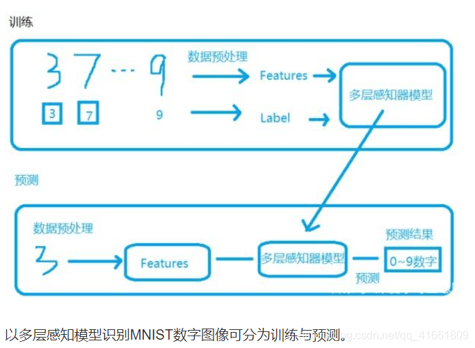
数据的预处理我们已经处理完了. 包含 数据集 输入(数字图像)的标准化 , label的one-hot encoding
我们将建立多层感知器模型 ,输入层 共有784 个神经元 ,hodden layer 有 256 个neure ,输出层用 10 个神经元 .
1 导入相关模块
from keras.models import Sequential
from keras.layers import Dense
2 建立 Sequence 模型
# 建立Sequential 模型
model = Sequential()
3 建立 "输入层" 和 "隐藏层"
使用 model,add() 方法加入 Dense 神经网络层 .
model.add(Dense(units=256,
          input_dim =784,
          keras_initializer='normal',
          activation='relu')
          )
| 参数 | 说明 |
| units =256 | 定义"隐藏层"神经元的个数为256 |
| input_dim | 设置输入层神经元个数为 784 |
| kernel_initialize='normal' | 使用正态分布的随机数初始化weight和bias |
| activation | 激励函数为 relu |
4 建立输出层
model.add(Dense(
    units=10,
    kernel_initializer='normal',
    activation='softmax'
))
| 参数 | 说明 |
| units | 定义"输出层"神经元个数为10 |
| kernel_initializer='normal' | 同上 |
| activation='softmax | 激活函数 softmax |
5 查看模型的摘要
print(model.summary())
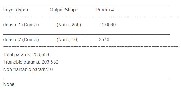
param 的计算是 上一次的神经元个数 * 本层神经元个数 + 本层神经元个数 .
1 定义训练方式
model.compile(loss='categorical_crossentropy' ,optimizer='adam',metrics=['accuracy'])
loss (损失函数) : 设置损失函数, 这里使用的是交叉熵 .
optimizer : 优化器的选择,可以让训练更快的收敛
metrics : 设置评估模型的方式是准确率
开始训练 2
train_history = model.fit(x=x_Train_normalize,y=y_TrainOneHot,validation_split=0.2 ,
                          epoch=10,batch_size=200,verbose=2)
使用 model.fit() 进行训练 , 训练过程会存储在 train_history 变量中 .
(1)输入训练数据参数
x = x_Train_normalize
y = y_TrainOneHot
(2)设置训练集和验证集的数据比例
validation_split=0.2 8 :2 = 训练集 : 验证集
(3) 设置训练周期 和 每一批次项数
epoch=10,batch_size=200
(4) 显示训练过程
verbose = 2
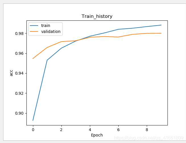
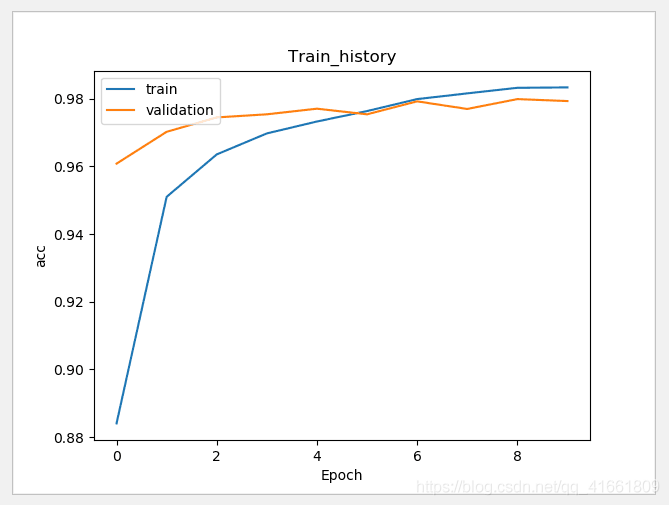
3 建立show_train_history 显示训练过程
def show_train_history(train_history,train,validation) :

    plt.plot(train_history.history[train])
    plt.plot(train_history.history[validation])
    plt.title("Train_history")
    plt.ylabel(train)
    plt.xlabel('Epoch')
    plt.legend(['train','validation'],loc='upper left')
    plt.show()

测试数据评估模型准确率
scores = model.evaluate(x_Test_normalize,y_TestOneHot)
print()
print('accuracy=',scores[1] )
accuracy= 0.9769
通过之前的步骤, 我们建立了模型, 并且完成了模型训练 ,准确率达到可以接受的 0.97 . 接下来我们将使用此模型进行预测.
1 执行预测
prediction = model.predict_classes(x_Test)
print(prediction)
result : [7 2 1 ... 4 5 6]
2 显示 10 项预测结果
plot_images_labels_prediction(x_test_image,y_test_label,prediction,idx=340)

我们可以看到 第一个数字 label 是 5 结果预测成 3 了.
上面我们在预测到第340 个测试集中的数字5 时 ,却被错误的预测成了 3 .如果想要更进一步的知道我们所建立的模型中哪些 数字的预测准确率更高 , 哪些数字会容忍混淆 .
混淆矩阵 也称为 误差矩阵.
1 使用Pandas 建立混淆矩阵 .
showMetrix = pd.crosstab(y_test_label,prediction,colnames=['label',],rownames=['predict'])
print(showMetrix)
label      0     1     2    3    4    5    6    7    8    9
predict
0        971     0     1    1    1    0    2    1    3    0
1          0  1124     4    0    0    1    2    0    4    0
2          5     0  1009    2    1    0    3    4    8    0
3          0     0     5  993    0    1    0    3    4    4
4          1     0     5    1  961    0    3    0    3    8
5          3     0     0   16    1  852    7    2    8    3
6          5     3     3    1    3    3  939    0    1    0
7          0     5    13    7    1    0    0  988    5    9
8          4     0     3    7    1    1    1    2  954    1
9          3     6     0   11    7    2    1    4    4  971
2 使用DataFrame
df = pd.DataFrame({'label ':y_test_label, 'predict':prediction})
print(df)
      label   predict
0          7        7
1          2        2
2          1        1
3          0        0
4          4        4
5          1        1
6          4        4
7          9        9
8          5        5
9          9        9
10         0        0
11         6        6
12         9        9
13         0        0
14         1        1
15         5        5
16         9        9
17         7        7
18         3        3
19         4        4
20         9        9
21         6        6
22         6        6
23         5        5
24         4        4
25         0        0
26         7        7
27         4        4
28         0        0
29         1        1
...      ...      ...
9970       5        5
9971       2        2
9972       4        4
9973       9        9
9974       4        4
9975       3        3
9976       6        6
9977       4        4
9978       1        1
9979       7        7
9980       2        2
9981       6        6
9982       5        6
9983       0        0
9984       1        1
9985       2        2
9986       3        3
9987       4        4
9988       5        5
9989       6        6
9990       7        7
9991       8        8
9992       9        9
9993       0        0
9994       1        1
9995       2        2
9996       3        3
9997       4        4
9998       5        5
9999       6        6
model.add(Dense(units=1000,
                input_dim=784,
                kernel_initializer='normal',
                activation='relu'))
hidden layer 神经元的增大,参数也增多了, 所以训练model的时间也变慢了.
加入 Dropout 功能避免过度拟合
# 建立Sequential 模型
model = Sequential()

model.add(Dense(units=1000,
                input_dim=784,
                kernel_initializer='normal',
                activation='relu'))
model.add(Dropout(0.5)) # 加入Dropout
model.add(Dense(units=10,
                kernel_initializer='normal',
                activation='softmax'))
训练的准确率 和 验证的准确率 差距变小了 .
建立多层感知器模型包含两层隐藏层
# 建立Sequential 模型
model = Sequential()
# 输入层 +" 隐藏层"1
model.add(Dense(units=1000,
                input_dim=784,
                kernel_initializer='normal',
                activation='relu'))
model.add(Dropout(0.5)) # 加入Dropout
# " 隐藏层"2
model.add(Dense(units=1000,
                kernel_initializer='normal',
                activation='relu'))
model.add(Dropout(0.5)) # 加入Dropout
# " 输出层"
model.add(Dense(units=10,
                kernel_initializer='normal',
                activation='softmax'))

print(model.summary())
代码:
import tensorflow as tf
import keras
import matplotlib.pyplot as plt
import numpy as np
from keras.utils import np_utils
from keras.datasets import mnist
from keras.models import Sequential
from keras.layers import Dense
from keras.layers import Dropout
import pandas as pd
import os

np.random.seed(10)
os.environ["CUDA_VISIBLE_DEVICES"] = "2"

(x_train_image ,y_train_label),(x_test_image,y_test_label) = mnist.load_data()

#
# print('train data = ' ,len(X_train_image)) #
# print('test data = ',len(X_test_image))

def plot_image(image):
    fig = plt.gcf()
    fig.set_size_inches(2,2)  # 设置图形的大小
    plt.imshow(image,cmap='binary') # 传入图像image ,cmap 参数设置为 binary ,以黑白灰度显示
    plt.show()
def plot_images_labels_prediction(images, labels,
                                  prediction, idx, num=10):
    fig = plt.gcf()
    fig.set_size_inches(12, 14)
    if num > 25: num = 25
    for i in range(0, num):
        ax = plt.subplot(5, 5, 1 + i)# 分成 5 X 5 个子图显示, 第三个参数表示第几个子图
        ax.imshow(images[idx], cmap='binary')
        title = "label=" + str(labels[idx])
        if len(prediction) > 0:
            title += ",predict=" + str(prediction[idx])

        ax.set_title(title, fOntsize=10)
        ax.set_xticks([])
        ax.set_yticks([])
        idx += 1
    plt.show()

def show_train_history(train_history,train,validation) :

    plt.plot(train_history.history[train])
    plt.plot(train_history.history[validation])
    plt.title("Train_history")
    plt.ylabel(train)
    plt.xlabel('Epoch')
    plt.legend(['train','validation'],loc='upper left')
    plt.show()

# plot_images_labels_prediction(x_train_image,y_train_image,[],0,10)
#
# plot_images_labels_prediction(x_test_image,y_test_image,[],0,10)
print("x_train_image : " ,len(x_train_image) , x_train_image.shape )
print("y_train_label : ", len(y_train_label) , y_train_label.shape)
# 将 image 以 reshape 转化

x_Train = x_train_image.reshape(60000,784).astype('float32')
x_Test = x_test_image.reshape(10000,784).astype('float32')

# print('x_Train : ' ,x_Train.shape)
# print('x_Test' ,x_Test.shape)
# 标准化
x_Test_normalize = x_Test/255
x_Train_normalize = x_Train/255

# print(x_Train_normalize[0]) # 训练集中的第一个数字的标准化
# 将训练集和测试集标签都进行独热码转化
y_TrainOneHot= np_utils.to_categorical(y_train_label)
y_TestOneHot= np_utils.to_categorical(y_test_label)
print(y_TrainOneHot[:5]) # 查看前5项的标签

# 建立Sequential 模型
model = Sequential()
model.add(Dense(units=1000,
                input_dim=784,
                kernel_initializer='normal',
                activation='relu'))
model.add(Dropout(0.5)) # 加入Dropout
# " 隐藏层"2
model.add(Dense(units=1000,
                kernel_initializer='normal',
                activation='relu'))
model.add(Dropout(0.5)) # 加入Dropout

model.add(Dense(units=10,
                kernel_initializer='normal',
                activation='softmax'))
print(model.summary())

# 训练方式
model.compile(loss='categorical_crossentropy' ,optimizer='adam',metrics=['accuracy'])
# 开始训练
train_history =model.fit(x=x_Train_normalize,
                         y=y_TrainOneHot,validation_split=0.2,
                         epochs=10, batch_size=200,verbose=2)

show_train_history(train_history,'acc','val_acc')
scores = model.evaluate(x_Test_normalize,y_TestOneHot)
print()
print('accuracy=',scores[1] )
prediction = model.predict_classes(x_Test)
print(prediction)
plot_images_labels_prediction(x_test_image,y_test_label,prediction,idx=340)
showMetrix = pd.crosstab(y_test_label,prediction,colnames=['label',],rownames=['predict'])
print(showMetrix)
df = pd.DataFrame({'label ':y_test_label, 'predict':prediction})
print(df)

#
#
# plot_image(x_train_image[0])
#
# print(y_train_image[0])
代码2:
import numpy as np
from keras.models import Sequential
from keras.layers import Dense , Dropout ,Deconv2D
from keras.utils import np_utils
from keras.datasets import mnist
from keras.optimizers import SGD
import os
os.environ["CUDA_VISIBLE_DEVICES"] = "2"
def load_data():
    (x_train,y_train),(x_test,y_test) = mnist.load_data()
    number = 10000
    x_train = x_train[0:number]
    y_train = y_train[0:number]

    x_train =x_train.reshape(number,28*28)
    x_test = x_test.reshape(x_test.shape[0],28*28)
    x_train = x_train.astype('float32')
    x_test = x_test.astype('float32')
    y_train = np_utils.to_categorical(y_train,10)
    y_test = np_utils.to_categorical(y_test,10)
    x_train = x_train/255
    x_test = x_test /255
    return (x_train,y_train),(x_test,y_test)
(x_train,y_train),(x_test,y_test) = load_data()

model = Sequential()
model.add(Dense(input_dim=28*28,units=689,activation='relu'))
model.add(Dropout(0.5))
model.add(Dense(units=689,activation='relu'))
model.add(Dropout(0.5))
model.add(Dense(units=689,activation='relu'))
model.add(Dropout(0.5))
model.add(Dense(output_dim=10,activation='softmax'))
model.compile(loss='categorical_crossentropy',optimizer='adam',metrics=['accuracy'])
model.fit(x_train,y_train,batch_size=10000,epochs=20)
res1 = model.evaluate(x_train,y_train,batch_size=10000)
print("\n Train Acc :",res1[1])
res2 = model.evaluate(x_test,y_test,batch_size=10000)
print("\n Test Acc :",res2[1])
以上为个人经验,希望能给大家一个参考,也希望大家多多支持。


 京公网安备 11010802041100号 | 京ICP备19059560号-4 | PHP1.CN 第一PHP社区 版权所有