篇首语:本文由编程笔记#小编为大家整理,主要介绍了难以定位heatmap.2组件相关的知识,希望对你有一定的参考价值。
我一直在努力定位我的heatmap.2输出的组件。
I found this old answer解释了@IanSudbery的元素定位是如何工作的,这看起来非常清楚,我认为它给了我理解我需要的东西,但我仍然没有抓住一些东西。
据我所知,这些元素基本上都放在了一个窗口的格子中,但它们的表现并不像我理解的那样。
这是我的代码和当前输出(在最底部是对图元素进行排序的感兴趣的点):
for(i in 1:length(ConditionsAbbr)) {
# creates its own colour palette
    my_palette <- colorRampPalette(c("snow", "yellow", "darkorange", "red"))(n = 399)
  # (optional) defines the colour breaks manually for a "skewed" colour transition
    col_breaks = c(seq(0,0.09,length=100),    #white 'snow'
                 seq(0.1,0.19,length=100), # for yellow
                 seq(0.2,0.29,length=100), # for orange 'darkorange'
                 seq(0.3,1,length=100))    # for red
  # creates a 5 x 5 inch image
  png(paste(SourceDir, "Heatmap_", ConditionsAbbr[i], "XYZ.png"),    # create PNG for the heat map
      width = 5*600,        # 5 x 600 pixels
      height = 5*600,
      res = 300,            # 300 pixels per inch
      pointsize = 8)        # smaller font size
  heatmap.2(ConditionsMtx[[ConditionsAbbr[i]]],
            cellnote = ConditionsMtx[[ConditionsAbbr[i]]],  # same data set for cell labels
            main =  paste(ConditionsAbbr[i], "XYZ"), # heat map title
            notecol="black",      # change font color of cell labels to black
            density.info="none",  # turns off density plot inside color legend
            trace="none",         # turns off trace lines inside the heat map
            margins =c(12,9),     # widens margins around plot
            col=my_palette,       # use on color palette defined earlier
            breaks=col_breaks,    # enable color transition at specified limits
            dendrogram="none",     # No dendogram
            srtCol = 0 ,        #correct angle of label numbers
            asp = 1 ,         #this overrides layout methinks and for some reason makes it square
            adjCol = c(NA, -35) ,
            adjRow = c(53, NA) ,
            keysize =  1.2 ,
            Colv = FALSE ,      #turn off column clustering
            Rowv =  FALSE ,    # turn off row clustering
            key.xlab = paste("Correlation") ,
            lmat = rbind( c(0, 3), c(2,1), c(0,4) ),
            lhei = c(0.9, 4, 0.5) )
  dev.off()               # close the PNG device
}
这给出了: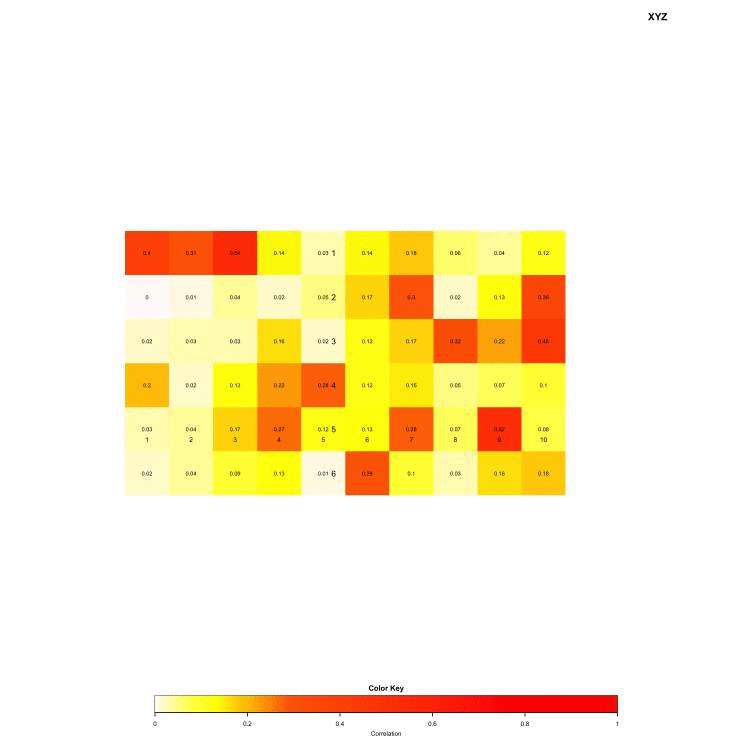
正如你所看到的,关键是矩阵的右边,矩阵,上面的标题和下面的键之间有大量的空白区域,甚至标题和矩阵都不在PNG的中心?
我觉得“我只会创建一个易于理解和编辑的3x3”,例如
        |        |
        |        |  (3)
        |        |
--------------------------
        |  (1)   |
   (2)  | Matrix |
        |        |
--------------------------
        |  (4)   |
        |  Key   |
        |        |
然后我可以摆脱白色空间,所以它更像是这样。
        |        |(3)
    ------------------
        |  (1)   |
     (2)| Matrix |
        |        |
    ------------------
        |(4) Key |
我这样做使用:
lmat = rbind( c(0, 0, 3), c(2, 1, 0), c(0, 4, 0) ),
            lhei = c(0.9, 4, 0.5) ,
            lwid = c(1, 4, 1))
这就是它的样子:
最好看到我的矩阵在中心,我的键仍然与我的矩阵右边对齐,我的标题是走丝绸之路东?更不用说所有多余的空白区域?
如何使这些对齐和一起移动,使图形组件紧密贴合在一起?
编辑:减少我的利润有助于减少空白,但它仍然过度。
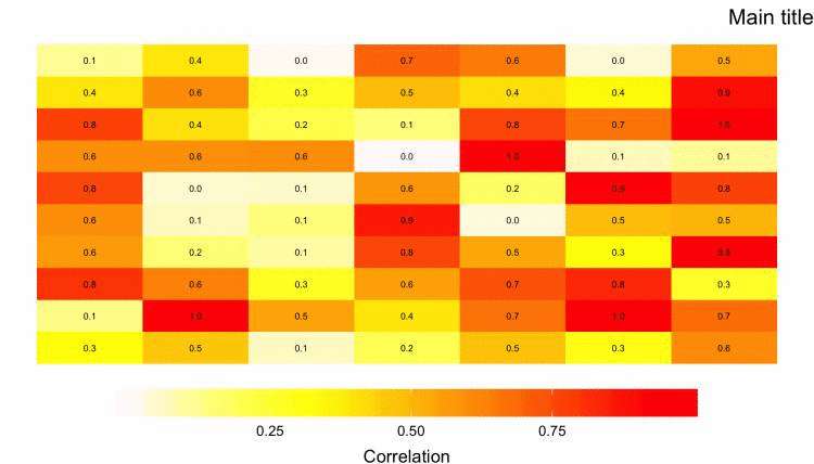
我不知道你是否对非基于heatmap.2的解决方案持开放态度。在我看来,ggplot提供了更大的灵活性,通过一些调整,您可以重现类似于您所展示的热像图,同时最大限度地绘制“不动产”并避免过多的空白。
如果你只是在寻找heatmap.2解决方案,我很高兴删除这篇文章。
除此之外,ggplot2解决方案可能如下所示:
首先,让我们生成一些样本数据
set.seed(2018)
df <- as_tibble(matrix(runif(7*10), ncol = 10), .name_repair = ~seq(1:10))
在绘图之前,我们需要将df从宽到长重塑
library(tidyverse)
df <- df %>%
    rowid_to_column("row") %>%
    gather(col, Correlation, -row) %>%
    mutate(col = as.integer(col))
然后去绘图
 ggplot(df, aes(row, col, fill = Correlation)) +
    geom_tile() +
    scale_fill_gradientn(colours = my_palette) +     # Use your custom colour palette
    theme_void() +                                   # Minimal theme
    labs(title = "Main title") +
    geom_text(aes(label = sprintf("%2.1f", Correlation)), size = 2) +
    theme(
        plot.title = element_text(hjust = 1),        # Right-aligned text
        legend.position="bottom") +                  # Legend at the bottom
    guides(fill = guide_colourbar(
        title.position = "bottom",                   # Legend title below bar
        barwidth = 25,                               # Extend bar length
        title.hjust = 0.5))
facet_wrap在网格布局中使用多个热图的示例首先,让我们生成更复杂的数据。
set.seed(2018)
df <- replicate(
    4,
    as_tibble(matrix(runif(7*10), ncol = 10), .name_repair = ~seq(1:10)), simplify = F) %>%
    setNames(., paste("data", 1:4, sep = "")) %>%
    map(~ .x %>% rowid_to_column("row") %>%
        gather(col, Correlation, -row) %>%
        mutate(col = as.integer(col))) %>%
    bind_rows(.id = "data")
然后,绘图与我们之前所做的相同,另外还有一个facet_wrap(~data, ncol = 2)声明
ggplot(df, aes(row, col, fill = Correlation)) +
    geom_tile() +
    scale_fill_gradientn(colours = my_palette) +     # Use your custom colour palette
    theme_void() +                                   # Minimal theme
    labs(title = "Main title") +
    geom_text(aes(label = sprintf("%2.1f", Correlation)), size = 2) +
    facet_wrap(~ data, ncol = 2) +
    theme(
        plot.title = element_text(hjust = 1),        # Right-aligned text
        legend.position="bottom") +                  # Legend at the bottom
    guides(fill = guide_colourbar(
        title.position = "bottom",                   # Legend title below bar
        barwidth = 25,                               # Extend bar length
        title.hjust = 0.5))
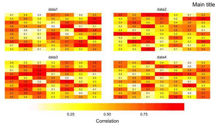
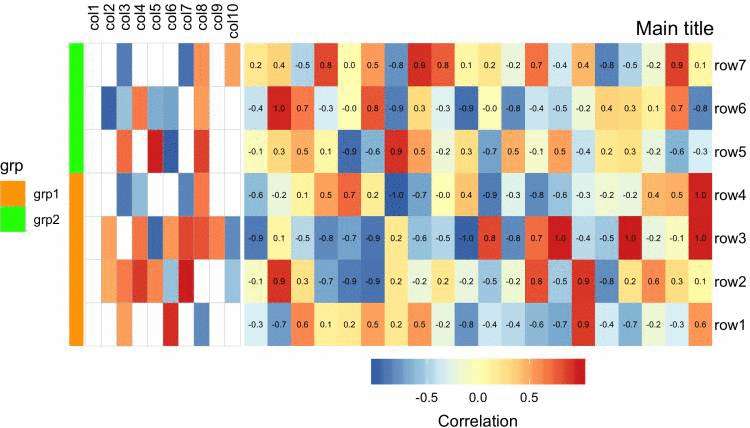
我认为看到我们可以走多远的复杂热图,与你的link to from the paper相似,这将是有趣/有趣的。
最后包含样本数据,因为这会占用一些空间。
我们首先构造三个不同的ggplot2绘图对象,显示主热图(gg3),另一个较小的热图(缺少值)(gg2),以及一个条形表示每行的组标签(gg1)。
gg3 <- ggplot(df.cor, aes(col, row, fill = Correlation)) +
    geom_tile() +
    scale_fill_distiller(palette = "RdYlBu") +
    theme_void() +
    labs(title = "Main title") +
    geom_text(aes(label = sprintf("%2.1f", Correlation)), size = 2) +
    scale_y_discrete(position = "right") +
    theme(
        plot.title = element_text(hjust = 1),
        legend.position="bottom",
        axis.text.y = element_text(color = "black", size = 10)) +
    guides(fill = guide_colourbar(
        title.position = "bottom",
        barwidth = 10,
        title.hjust = 0.5))
gg2 <- ggplot(df.flag, aes(col, row, fill = Correlation)) +
    geom_tile(colour = "grey") +
    scale_fill_distiller(palette = "RdYlBu", guide = F, na.value = "white") +
    theme_void() +
    scale_x_discrete(position = "top") +
    theme(
        axis.text.x = element_text(color = "black", size = 10, angle = 90, hjust = 1, vjust = 0.5))
gg1 <- ggplot(df.bar, aes(1, row, fill = grp)) +
    geom_tile() +
    scale_fill_manual(values = c("grp1" = "orange", "grp2" = "green")) +
    theme_void() +
    theme(legend.position = "left")
我们现在可以使用egg::ggarrange定位所有三个图,使y轴范围对齐。
library(egg)
ggarrange(gg1, gg2, gg3, ncol = 3, widths = c(0.1, 1, 3))
library(tidyverse)
set.seed(2018)
nrow <- 7
ncol <- 20
df.cor <- matrix(runif(nrow * ncol, min = -1, max = 1), nrow = nrow) %>%
    as_tibble(.name_repair = ~seq(1:ncol)) %>%
    rowid_to_column("row") %>%
    gather(col, Correlation, -row) %>%
    mutate(
        row = factor(
            paste("row", row, sep = ""),
            levels = paste("row", 1:nrow, sep = "")),
        col = factor(
            paste("col", col, sep = ""),
            levels = paste("col", 1:ncol, sep = "")))
nrow <- 7
ncol <- 10
df.flag <- matrix(runif(nrow * ncol, min = -1, max = 1), nrow = nrow) %>%
    as_tibble(.name_repair = ~seq(1:ncol)) %>%
    rowid_to_column("row") %>%
    gather(col, Correlation, -row) %>%
    mutate(
        row = factor(
            paste("row", row, sep = ""),
            levels = paste("row", 1:nrow, sep = "")),
        col = factor(
            paste("col", col, sep = ""),
            levels = paste("col", 1:ncol, sep = ""))) %>%
    mutate(Correlation = ifelse(abs(Correlation) <0.5, NA, Correlation))
df.bar <- data.frame(
    row = 1:nrow,
    grp = paste("grp", c(rep(1, nrow - 3), rep(2, 3)), sep = "")) %>%
    mutate(
        row = factor(
            paste("row", row, sep = ""),
            levels = paste("row", 1:nrow, sep = "")))
以下是我为获得结果所做的最终更改,但是,如果您不太投资于热图,我建议您使用Maurits Evers的建议。不要忽视我对图像尺寸所做的更改。
# creates my own colour palette
my_palette <- colorRampPalette(c("snow", "yellow", "darkorange", "red"))(n = 399)
# (optional) defines the colour breaks manually for a "skewed" colour transition
col_breaks = c(seq(0,0.09,length=100), #white 'snow'
seq(0.1,0.19,length=100), # for yellow
seq(0.2,0.29,length=100), # for orange 'darkorange'
seq(0.3,1,length=100)) # for red
# creates an image
png(paste(SourceDir, "Heatmap_XYZ.png" )
# create PNG for the heat map
width = 5*580, # 5 x 580 pixels
height = 5*420, # 5 x 420 pixels
res = 300, # 300 pixels per inch
pointsize =11) # smaller font size
heatmap.2(ConditionsMtx[[ConditionsAbbr[i]]],
cellnote = ConditionsMtx[[ConditionsAbbr[i]]], # same data set for cell labels
main = "XYZ", # heat map title
notecol="black", # change font color of cell labels to black
density.info="none", # turns off density plot inside color legend
trace="none", # turns off trace lines inside the heat map
margins=c(0,0), # widens margins around plot
col=my_palette, # use on color palette defined earlier
breaks=col_breaks, # enable color transition at specified limits
dendrogram="none", # only draw a row dendrogra


 京公网安备 11010802041100号 | 京ICP备19059560号-4 | PHP1.CN 第一PHP社区 版权所有