%% 第9章 形态学处理
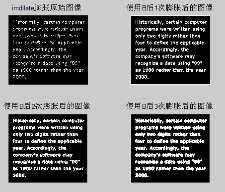
%% imdilate膨胀
clc
clear
A1=imread(\'.\images\dipum_images_ch09\Fig0906(a)(broken-text).tif\');
info=imfinfo(\'.\images\dipum_images_ch09\Fig0906(a)(broken-text).tif\')
B=[0 1 0
1 1 1
0 1 0];
A2=imdilate(A1,B);%图像A1被结构元素B膨胀
A3=imdilate(A2,B);
A4=imdilate(A3,B);
subplot(221),imshow(A1);
title(\'imdilate膨胀原始图像\');
subplot(222),imshow(A2);
title(\'使用B后1次膨胀后的图像\');
subplot(223),imshow(A3);
title(\'使用B后2次膨胀后的图像\');
subplot(224),imshow(A4);
title(\'使用B后3次膨胀后的图像\');
27%imdilate图像膨胀处理过程运行结果如下:
 %% imerode腐蚀
clc
clear
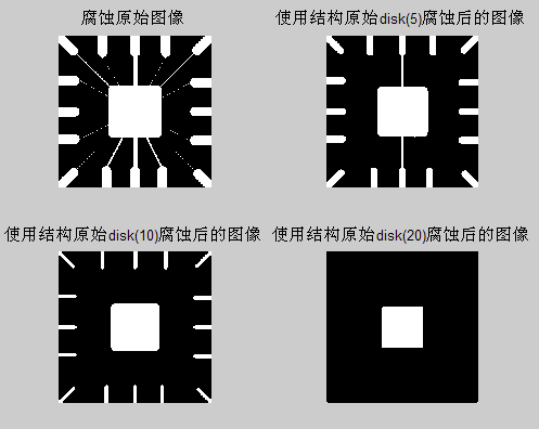
A1=imread(\'.\images\dipum_images_ch09\Fig0908(a)(wirebond-mask).tif\');
subplot(221),imshow(A1);
title(\'腐蚀原始图像\');
%strel函数的功能是运用各种形状和大小构造结构元素
se1=strel(\'disk\',5);%这里是创建一个半径为5的平坦型圆盘结构元素
A2=imerode(A1,se1);
subplot(222),imshow(A2);
title(\'使用结构原始disk(5)腐蚀后的图像\');
se2=strel(\'disk\',10);
A3=imerode(A1,se2);
subplot(223),imshow(A3);
title(\'使用结构原始disk(10)腐蚀后的图像\');
se3=strel(\'disk\',20);
A4=imerode(A1,se3);
subplot(224),imshow(A4);
title(\'使用结构原始disk(20)腐蚀后的图像\');
%图像腐蚀处理过程运行结果如下:
%% imerode腐蚀
clc
clear
A1=imread(\'.\images\dipum_images_ch09\Fig0908(a)(wirebond-mask).tif\');
subplot(221),imshow(A1);
title(\'腐蚀原始图像\');
%strel函数的功能是运用各种形状和大小构造结构元素
se1=strel(\'disk\',5);%这里是创建一个半径为5的平坦型圆盘结构元素
A2=imerode(A1,se1);
subplot(222),imshow(A2);
title(\'使用结构原始disk(5)腐蚀后的图像\');
se2=strel(\'disk\',10);
A3=imerode(A1,se2);
subplot(223),imshow(A3);
title(\'使用结构原始disk(10)腐蚀后的图像\');
se3=strel(\'disk\',20);
A4=imerode(A1,se3);
subplot(224),imshow(A4);
title(\'使用结构原始disk(20)腐蚀后的图像\');
%图像腐蚀处理过程运行结果如下:
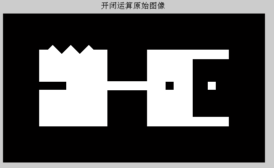
 %% 开运算和闭运算
clc
clear
f=imread(\'.\images\dipum_images_ch09\Fig0910(a)(shapes).tif\');
%se=strel(\'square\',5\');%方型结构元素
se=strel(\'disk\',5\');%圆盘型结构元素
imshow(f);%原图像
title(\'开闭运算原始图像\')
61%运行结果如下:
%% 开运算和闭运算
clc
clear
f=imread(\'.\images\dipum_images_ch09\Fig0910(a)(shapes).tif\');
%se=strel(\'square\',5\');%方型结构元素
se=strel(\'disk\',5\');%圆盘型结构元素
imshow(f);%原图像
title(\'开闭运算原始图像\')
61%运行结果如下:
 %开运算数学上是先腐蚀后膨胀的结果
%开运算的物理结果为完全删除了不能包含结构元素的对象区域,平滑
%了对象的轮廓,断开了狭窄的连接,去掉了细小的突出部分
fo=imopen(f,se);%直接开运算
figure,subplot(221),imshow(fo);
title(\'直接开运算\');
%闭运算在数学上是先膨胀再腐蚀的结果
%闭运算的物理结果也是会平滑对象的轮廓,但是与开运算不同的是,闭运算
%一般会将狭窄的缺口连接起来形成细长的弯口,并填充比结构元素小的洞
fc=imclose(f,se);%直接闭运算
subplot(222),imshow(fc);
title(\'直接闭运算\');
foc=imclose(fo,se);%先开后闭运算
subplot(223),imshow(foc);
title(\'先开后闭运算\');
fco=imopen(fc,se);%先闭后开运算
subplot(224),imshow(fco);
title(\'先闭后开运算\');
84%开闭运算结果如下:
%开运算数学上是先腐蚀后膨胀的结果
%开运算的物理结果为完全删除了不能包含结构元素的对象区域,平滑
%了对象的轮廓,断开了狭窄的连接,去掉了细小的突出部分
fo=imopen(f,se);%直接开运算
figure,subplot(221),imshow(fo);
title(\'直接开运算\');
%闭运算在数学上是先膨胀再腐蚀的结果
%闭运算的物理结果也是会平滑对象的轮廓,但是与开运算不同的是,闭运算
%一般会将狭窄的缺口连接起来形成细长的弯口,并填充比结构元素小的洞
fc=imclose(f,se);%直接闭运算
subplot(222),imshow(fc);
title(\'直接闭运算\');
foc=imclose(fo,se);%先开后闭运算
subplot(223),imshow(foc);
title(\'先开后闭运算\');
fco=imopen(fc,se);%先闭后开运算
subplot(224),imshow(fco);
title(\'先闭后开运算\');
84%开闭运算结果如下:
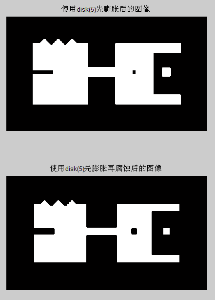
%先膨胀再腐蚀
fse=imdilate(f,se);%膨胀
%gcf为得到当前图像的句柄,当前图像是指例如PLOT,TITLE,SURF等
%get函数为得到物体的属性,get(0,\'screensize\')为返回所有物体screensize属性值
%set函数为设置物体的属性
figure,set(gcf,\'outerposition\',get(0,\'screensize\'));%具体目的是设置当前窗口的大小
subplot(211),imshow(fse);
title(\'使用disk(5)先膨胀后的图像\');
fes=imerode(fse,se);
subplot(212),imshow(fes);
title(\'使用disk(5)先膨胀再腐蚀后的图像\');
99%先膨胀后腐蚀图像如下:
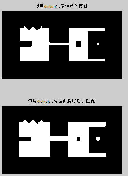
%先腐蚀再膨胀
fse=imerode(f,se);
figure,set(gcf,\'outerposition\',get(0,\'screensize\'))
subplot(211),imshow(fse);
title(\'使用disk(5)先腐蚀后的图像\');
fes=imdilate(fse,se);
subplot(212),imshow(fes);
title(\'使用disk(5)先腐蚀再膨胀后的图像\');
110%先腐蚀后膨胀的图像如下:
%% imopen imclose在指纹上的应用
clc
clear
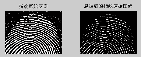
f=imread(\'.\images\dipum_images_ch09\Fig0911(a)(noisy-fingerprint).tif\');
se=strel(\'square\',3);%边长为3的方形结构元素
subplot(121),imshow(f);
title(\'指纹原始图像\');
A=imerode(f,se);%腐蚀
subplot(122),imshow(A);
title(\'腐蚀后的指纹原始图像\');
123%指纹原始图像和腐蚀后的图像结果如下:
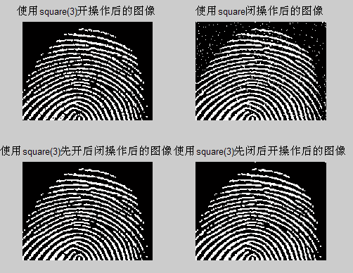
fo=imopen(f,se);
figure,subplot(221),imshow(fo);
title(\'使用square(3)开操作后的图像\');
fc=imclose(f,se);
subplot(222),imshow(fc);
title(\'使用square闭操作后的图像\');
foc=imclose(fo,se);
subplot(223),imshow(foc);
title(\'使用square(3)先开后闭操作后的图像\')
fco=imopen(fc,se);
subplot(224),imshow(fco);
title(\'使用square(3)先闭后开操作后的图像\');
140%指纹图像开闭操作过程结果如下:
%% bwhitmiss击中或击不中变换
clc
clear
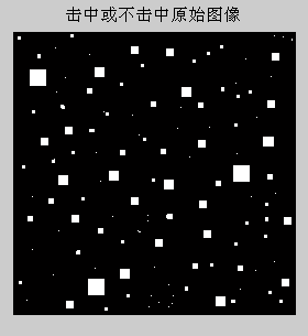
f=imread(\'.\images\dipum_images_ch09\Fig0913(a)(small-squares).tif\');
imshow(f);
title(\'击中或不击中原始图像\');
148%击中或不击中原始图像显示结果如下:
 B1=strel([0 0 0;0 1 1;0 1 0]);%击中:要求击中所有1的位置
B2=strel([1 1 1;1 0 0;1 0 0]);%击不中,要求击不中所有1的位置
B3=strel([0 1 0;1 1 1;0 1 0]);%击中
B4=strel([1 0 1;0 0 0;0 0 0]);%击不中
B5=strel([0 0 0;0 1 0;0 0 0]);%击中
B6=strel([1 1 1;1 0 0;1 0 0]);%击不中
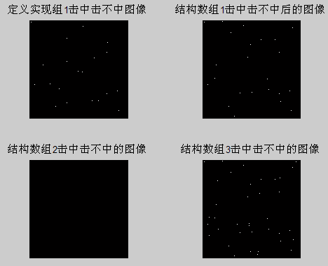
g=imerode(f,B1)&imerode(~f,B2)%利用定义来实现击中或击不中
figure,subplot(221),imshow(g);
title(\'定义实现组1击中击不中图像\');
g1=bwhitmiss(f,B1,B2);
subplot(222),imshow(g1);
title(\'结构数组1击中击不中后的图像\');
g2=bwhitmiss(f,B3,B4);
subplot(223),imshow(g2);
title(\'结构数组2击中击不中的图像\');
g3=bwhitmiss(f,B5,B6);
subplot(224),imshow(g3);
title(\'结构数组3击中击不中的图像\');
172%击中击不中变换后图像如下:
B1=strel([0 0 0;0 1 1;0 1 0]);%击中:要求击中所有1的位置
B2=strel([1 1 1;1 0 0;1 0 0]);%击不中,要求击不中所有1的位置
B3=strel([0 1 0;1 1 1;0 1 0]);%击中
B4=strel([1 0 1;0 0 0;0 0 0]);%击不中
B5=strel([0 0 0;0 1 0;0 0 0]);%击中
B6=strel([1 1 1;1 0 0;1 0 0]);%击不中
g=imerode(f,B1)&imerode(~f,B2)%利用定义来实现击中或击不中
figure,subplot(221),imshow(g);
title(\'定义实现组1击中击不中图像\');
g1=bwhitmiss(f,B1,B2);
subplot(222),imshow(g1);
title(\'结构数组1击中击不中后的图像\');
g2=bwhitmiss(f,B3,B4);
subplot(223),imshow(g2);
title(\'结构数组2击中击不中的图像\');
g3=bwhitmiss(f,B5,B6);
subplot(224),imshow(g3);
title(\'结构数组3击中击不中的图像\');
172%击中击不中变换后图像如下:
%%makelut
clc
clear
f=inline(\'sum(x(:))>=3\');%inline是用来定义局部函数的
lut2=makelut(f,2)%为函数f构造一个接收2*2矩阵的查找表
lut3=makelut(f,3)
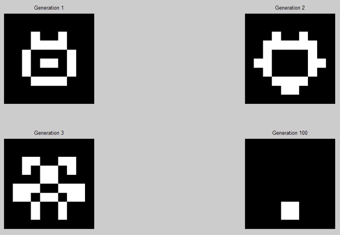
%% Conway生命游戏
clc
clear
lut=makelut(@conwaylaws,3);
bw1= [0 0 0 0 0 0 0 0 0 0
0 0 0 0 0 0 0 0 0 0
0 0 0 1 0 0 1 0 0 0
0 0 0 1 1 1 1 0 0 0
0 0 1 0 0 0 0 1 0 0
0 0 1 0 1 1 0 1 0 0
0 0 1 0 0 0 0 1 0 0
0 0 0 1 1 1 1 0 0 0
0 0 0 0 0 0 0 0 0 0
0 0 0 0 0 0 0 0 0 0 ];
subplot(221),imshow(bw1,\'InitialMagnification\',\'fit\');
title(\'Generation 1\');
bw2=applylut(bw1,lut);
subplot(222),imshow(bw2,\'InitialMagnification\',\'fit\'),
title(\'Generation 2\');
bw3=applylut(bw2,lut);
subplot(223),imshow(bw3,\'InitialMagnification\',\'fit\');
title(\'Generation 3\');
temp=bw1;
for i=2:100
bw100=applylut(temp,lut);
temp=bw100;
end
subplot(224),imshow(bw100,\'InitialMagnification\',\'fit\')
title(\'Generation 100\');
214%显示Generation结果如下:
%% getsequence
clc
clear
se=strel(\'diamond\',5)
decomp=getsequence(se)%getsequence函数为得到分解的strel序列
decomp(1)
decomp(2)
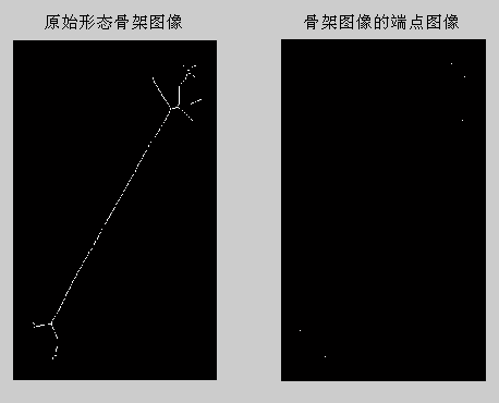
%% endpoints
clc
clear
f1=imread(\'.\images\dipum_images_ch09\Fig0914(a)(bone-skel).tif\');
subplot(121),imshow(f1);
title(\'原始形态骨架图像\');
g1=endpoints(f1);
%set(gcf,\'outerposition\',get(0,\'screensize\'));%运行完后自动生成最大的窗口
subplot(122),imshow(g1);
title(\'骨架图像的端点图像\');
%骨架头像端点检测头像如下:
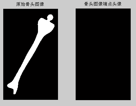
f2=imread(\'.\images\dipum_images_ch09\Fig0916(a)(bone).tif\');
figure,subplot(121),imshow(f2);
title(\'原始骨头图像\');
g2=endpoints(f2);
subplot(122),imshow(g2);
title(\'骨头图像端点头像\');%结果是没有端点
245%骨头头像端点检测图像如下:
%% bwmorph组合常见形态学之细化
clc
clear
f=imread(\'.\images\dipum_images_ch09\Fig0911(a)(noisy-fingerprint).tif\');
subplot(221),imshow(f);
title(\'指纹图像细化原图\');

g1=bwmorph(f,\'thin\',1);
subplot(222),imshow(g1);
title(\'指纹图像细化原图\');

g2=bwmorph(f,\'thin\',2);
subplot(223),imshow(g2);
title(\'指纹图像细化原图\');

g3=bwmorph(f,\'thin\',Inf);
subplot(224),imshow(g3);
title(\'指纹图像细化原图\');
265%指纹图像细化过程显示如下:

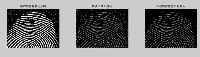
%% bwmorph组合常见形态学之骨骼化
clc
clear
f=imread(\'.\images\dipum_images_ch09\Fig0911(a)(noisy-fingerprint).tif\');
subplot(131),imshow(f);
title(\'指纹图像骨骼化原图\');
fs=bwmorph(f,\'skel\',Inf);
subplot(132),imshow(fs);
title(\'指纹图像骨骼化\');
for k=1:5
fs=fs&~endpoints(fs);
end
subplot(133),imshow(fs);
title(\'指纹图像修剪后骨骼话\');
283%指纹图像骨骼化过程显示:
%% 使用函数bwlabel标注连通分量
clc
clear
f=imread(\'.\images\dipum_images_ch09\Fig0917(a)(ten-objects).tif\');
imshow(f),title(\'标注连通分量原始图像\');
290%其结果显示如下:
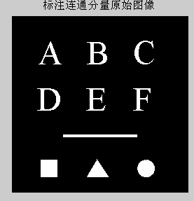 [L,n]=bwlabel(f);%L为标记矩阵,n为找到连接分量的总数
[r,c]=find(L==3);%返回第3个对象所有像素的行索引和列索引
rbar=mean(r);
cbar=mean(c);
figure,imshow(f)
hold on%保持当前图像使其不被刷新
for k=1:n
[r,c]=find(L==k);
rbar=mean(r);
cbar=mean(c);
plot(cbar,rbar,\'Marker\',\'o\',\'MarkerEdgeColor\',\'k\',...
\'MarkerFaceColor\',\'k\',\'MarkerSize\',10);%这个plot函数用法不是很熟悉
plot(cbar,rbar,\'Marker\',\'*\',\'MarkerFaceColor\',\'w\');%其中的marker为标记
end
title(\'标记所有对象质心后的图像\');
[L,n]=bwlabel(f);%L为标记矩阵,n为找到连接分量的总数
[r,c]=find(L==3);%返回第3个对象所有像素的行索引和列索引
rbar=mean(r);
cbar=mean(c);
figure,imshow(f)
hold on%保持当前图像使其不被刷新
for k=1:n
[r,c]=find(L==k);
rbar=mean(r);
cbar=mean(c);
plot(cbar,rbar,\'Marker\',\'o\',\'MarkerEdgeColor\',\'k\',...
\'MarkerFaceColor\',\'k\',\'MarkerSize\',10);%这个plot函数用法不是很熟悉
plot(cbar,rbar,\'Marker\',\'*\',\'MarkerFaceColor\',\'w\');%其中的marker为标记
end
title(\'标记所有对象质心后的图像\');

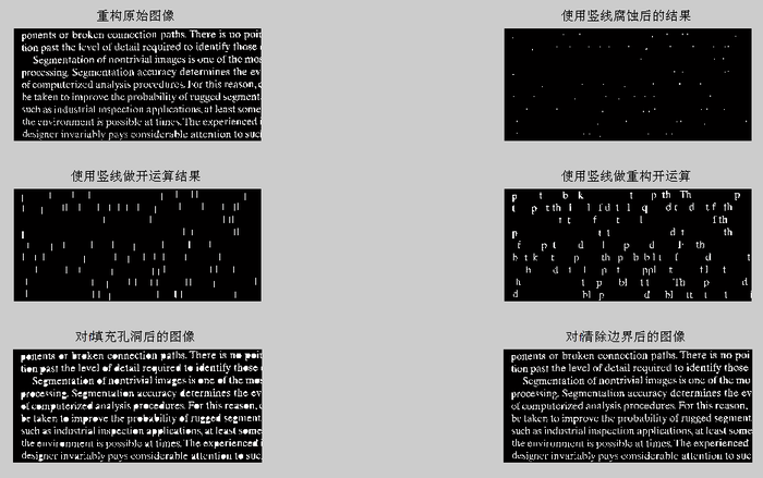
%% 由重构做开运算
clc
clear
f=imread(\'.\images\dipum_images_ch09\Fig0922(a)(book-text).tif\');
subplot(321),imshow(f);
title(\'重构原始图像\');

fe=imerode(f,ones(51,1));%竖线腐蚀
subplot(322),imshow(fe);
title(\'使用竖线腐蚀后的结果\');

fo=imopen(f,ones(51,1));%竖线做开运算
subplot(323),imshow(fo);
title(\'使用竖线做开运算结果\');

fobr=imreconstruct(fe,f);%fe做标记
subplot(324),imshow(fobr);
title(\'使用竖线做重构开运算\');

ff=imfill(f,\'holes\');%对f进行孔洞填充
subplot(325),imshow(ff);
title(\'对f填充孔洞后的图像\');

fc=imclearborder(f,8);%清除边界,2维8邻接
subplot(326),imshow(fc);
title(\'对f清除边界后的图像\');
336%图像重构过程显示如下:
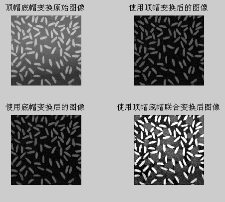
%% 使用顶帽变换和底帽变换
clc
clear
f=imread(\'.\images\dipum_images_ch09\Fig0926(a)(rice).tif\');
subplot(221),imshow(f);
title(\'顶帽底帽变换原始图像\');
se=strel(\'disk\',10);%产生结构元素
%顶帽变换是指原始图像减去其开运算的图像
%而开运算可用于补偿不均匀的背景亮度,所以用一个大的结构元素做开运算后
%然后用原图像减去这个开运算,就得到了背景均衡的图像,这也叫做是图像的顶帽运算
f1=imtophat(f,se);%使用顶帽变换
subplot(222),imshow(f1);
title(\'使用顶帽变换后的图像\');
%底帽变换是原始图像减去其闭运算后的图像
f2=imbothat(imcomplement(f),se);%使用底帽变换,为什么原图像要求补呢?
%f2=imbothat(f,se);%使用底帽变换
subplot(223),imshow(f2);
title(\'使用底帽变换后的图像\');
%顶帽变换和底帽变换联合起来用,用于增加对比度
f3=imsubtract(imadd(f,imtophat(f,se)),imbothat(f,se));%里面参数好像不合理?
subplot(224),imshow(f3);
title(\'使用顶帽底帽联合变换后图像\');
363%顶帽底帽变换过程图像如下:
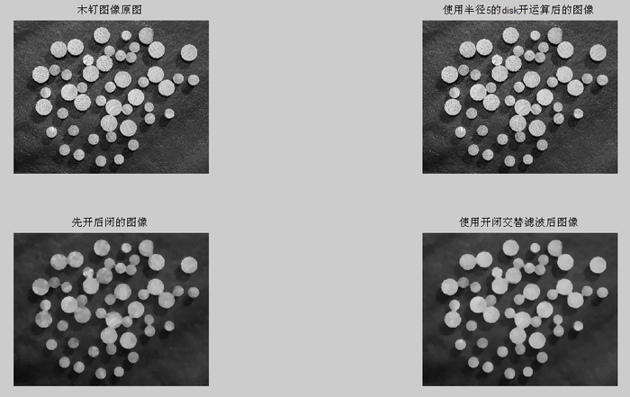
%%使用开运算和闭运算做形态学平滑
%由于开运算可以除去比结构元素更小的明亮细节,闭运算可以除去比结构元素更小的暗色细节
%所以它们经常组合起来一起进行平滑图像并去除噪声
clc
clear
f=imread(\'.\images\dipum_images_ch09\Fig0925(a)(dowels).tif\');
subplot(221),imshow(f);
title(\'木钉图像原图\');
se=strel(\'disk\',5);%disk其实就是一个八边形
fo=imopen(f,se);%经过开运算
subplot(222),imshow(f);
title(\'使用半径5的disk开运算后的图像\');
foc=imclose(fo,se);
subplot(223),imshow(foc);
title(\'先开后闭的图像\');
fasf=f;
for i=2:5
se=strel(\'disk\',i);
fasf=imclose(imopen(fasf,se),se);
end
subplot(224),imshow(fasf);
title(\'使用开闭交替滤波后图像\');
390%使用开运算和闭运算做形态学平滑结果如下:
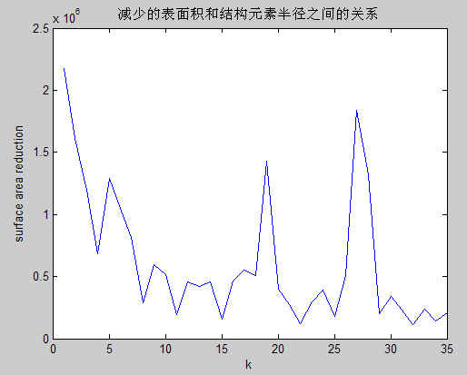
%% 颗粒分析
clc
clear
f=imread(\'.\images\dipum_images_ch09\Fig0925(a)(dowels).tif\');
sumpixels=zeros(1,36);
for k=0:35
se=strel(\'disk\',k);
fo=imopen(f,se);
sumpixels(k+1)=sum(fo(:));
end
%可以看到,连续开运算之间的表面积会减少
plot(0:35,sumpixels),xlabel(\'k\'),ylabel(\'surface area\');
title(\'表面积和结构元素半径之间的关系\');
407%其运算结果如下:
 figure,plot(-diff(sumpixels));%diff()函数为差分或者近似倒数,即相邻2个之间的差值
xlabel(\'k\'),ylabel(\'surface area reduction\');
title(\'减少的表面积和结构元素半径之间的关系\');
412%其运算结果如下:
figure,plot(-diff(sumpixels));%diff()函数为差分或者近似倒数,即相邻2个之间的差值
xlabel(\'k\'),ylabel(\'surface area reduction\');
title(\'减少的表面积和结构元素半径之间的关系\');
412%其运算结果如下:
%% 使用重构删除复杂图像的背景
clc
clear
f=imread(\'.\images\dipum_images_ch09\Fig0930(a)(calculator).tif\');
subplot(221),imshow(f);
title(\'灰度级重构原图像\');
f_obr=imreconstruct(imerode(f,ones(1,71)),f);
subplot(222),imshow(f_obr);
title(\'经开运算重构图\');
f_o=imopen(f,ones(1,71));
subplot(223),imshow(f_o);
title(\'经开运算后图\');
f_thr=imsubtract(f,f_obr);
subplot(224),imshow(f_thr);
title(\'顶帽运算重构图\')
432%使用重构删除复杂图像的背景1:
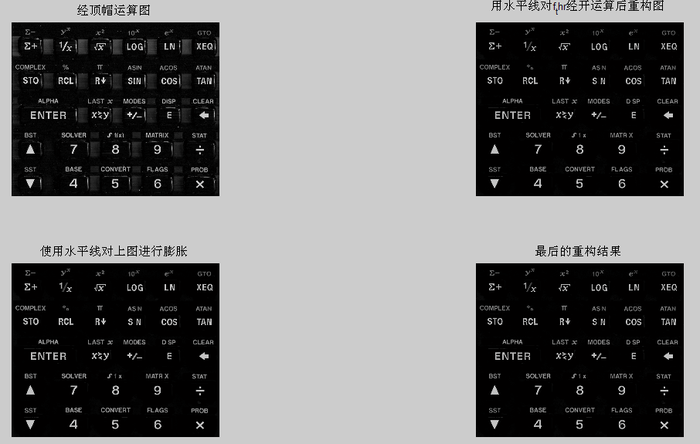
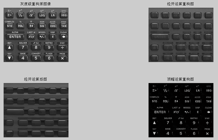 f_th=imsubtract(f,f_o)
figure,subplot(221),imshow(f_th);
title(\'经顶帽运算图\');
g_obr=imreconstruct(imerode(f_thr,ones(1,11)),f_thr);
subplot(222),imshow(g_obr);
title(\'用水平线对f_thr经开运算后重构图\');
g_obrd=imdilate(g_obr,ones(1,2));
subplot(223),imshow(g_obrd);
title(\'使用水平线对上图进行膨胀\');
f2=imreconstruct(min(g_obrd,f_thr),f_thr);
subplot(224),imshow(f2);
title(\'最后的重构结果\');
449%使用重构删除复杂图像的背景2:
f_th=imsubtract(f,f_o)
figure,subplot(221),imshow(f_th);
title(\'经顶帽运算图\');
g_obr=imreconstruct(imerode(f_thr,ones(1,11)),f_thr);
subplot(222),imshow(g_obr);
title(\'用水平线对f_thr经开运算后重构图\');
g_obrd=imdilate(g_obr,ones(1,2));
subplot(223),imshow(g_obrd);
title(\'使用水平线对上图进行膨胀\');
f2=imreconstruct(min(g_obrd,f_thr),f_thr);
subplot(224),imshow(f2);
title(\'最后的重构结果\');
449%使用重构删除复杂图像的背景2:
形态学这一章很有用,因为它还可以应用在图像分割中。
原文链接:http://blog.csdn.net/yangyangyang20092010/article/details/8289572
发表于
2015-11-14 15:35
hope1314
阅读(5369)
评论(0)
编辑
收藏
举报


 京公网安备 11010802041100号